The cluster categories:
Knowns with PFAM (Ks): ORF clusters that have been annotated with a PFAM domains of known function.
Knowns without PFAMs (KWPs): clusters that have a known function, but do not contain PFAM annotations.
Genomic Unknowns (GUs): ORF clusters that have an unknown function (e.g. DUF, hypothetical protein) but are found in sequenced or draft-genomes, or in population genomes (or Metagenome Assembled Genomes).
Environmental Unknowns (EUs): ORF clusters of unknown function that are not found in sequenced or draft genomes, but only in environmental metagenomes.
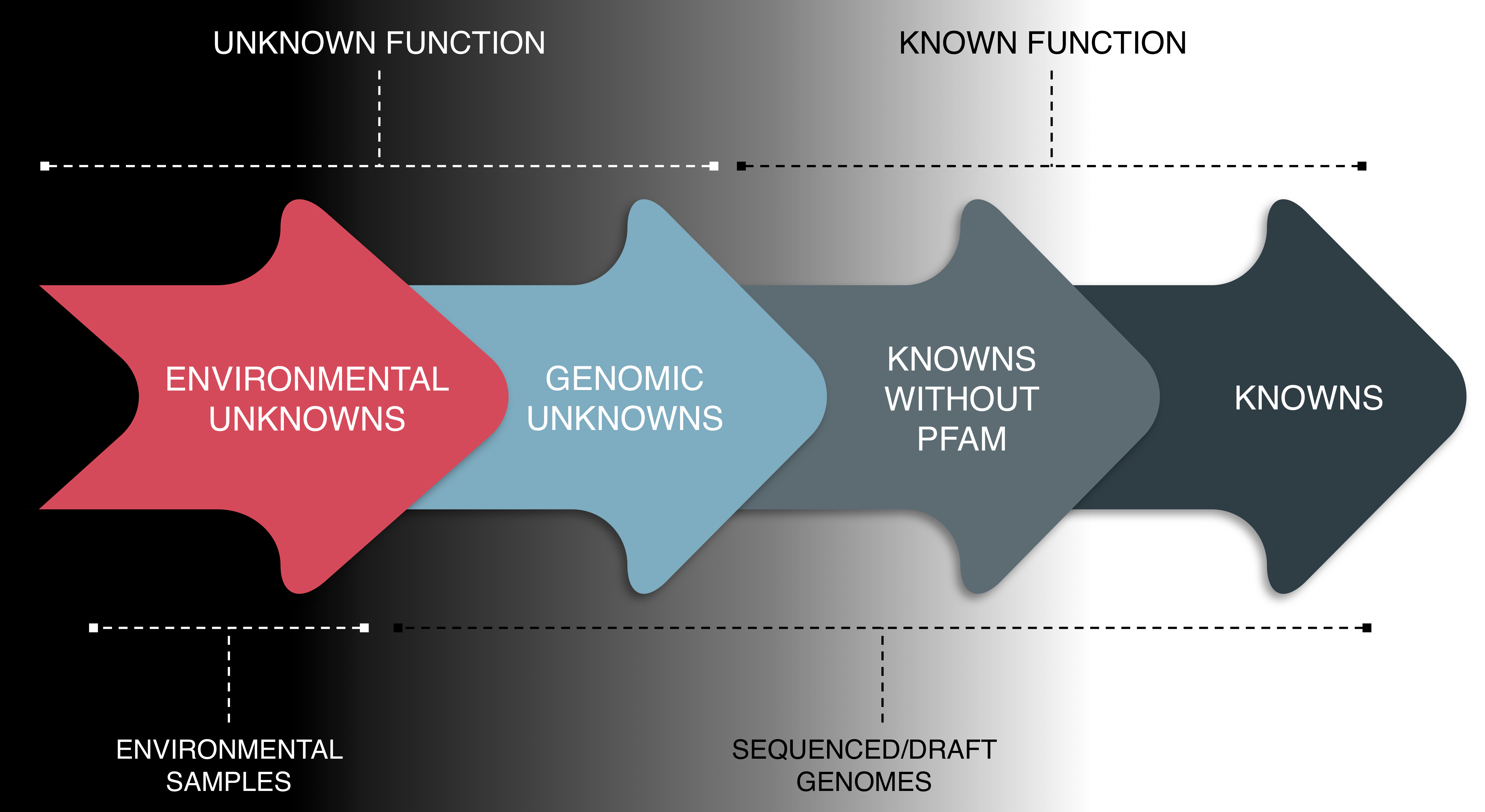
Cluster categories overview.
Number of clusters and ORFs on the different categories
| K | KWP | GU | EU | Total | |
|---|---|---|---|---|---|
| Clusters | 1,050,166 | 632,453 | 1,121,809 | 135,829 | 2,940,257 |
| ORFs | 172,147,128 | 30,601,694 | 54,052,275 | 3,341,257 | 260,142,354 |
Cluster category information and statisitcs
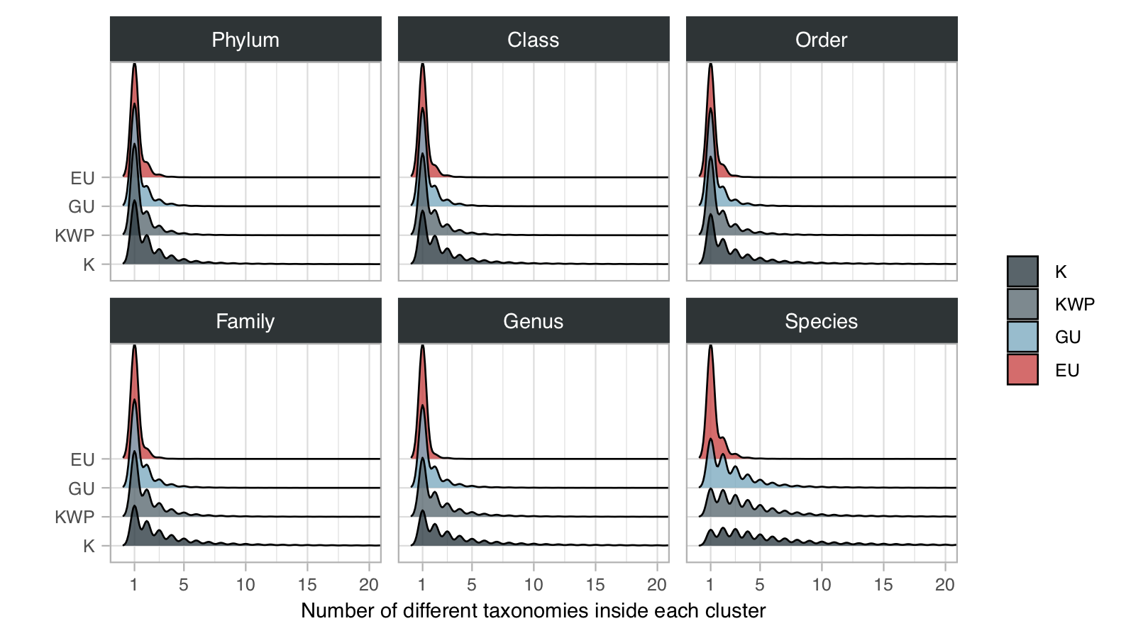
1. Taxonomy (and cluster taxonomic homogeneity)
Methods
To retrieve the taxonomic composition of our clusters we applied the MMseqs2 taxonomy program [1], which allows computing the lowest common ancestor through the implementation of the 2bLCA protocol [2]. For each cluster category we searched the ORFs against the Uniprot entries (UniProtKB release 2018_04), annotated with the NCBI taxonomy, using the MMseqs2 (version: b43de8b7559a3b45c8e5e9e02cb3023dd339231a) software taxonomy workflow, as explained here. “By identifying homologs through searches with taxonomy annotated reference databases, MMseqs2 can compute the lowest common ancestor. This lowest common ancestor is a robust taxonomic label for unknown sequences. MMseqs2 implements the 2bLCA protocol with –lca-mode 2 for choosing a robust LCA. The LCA implementation is based on the Go implementation of blast2lca software on GitHub. It implements the LCA computation efficiently through Range Minimum Queries through an dynamic programming approach.”
MMseqs2 needs the NCBI taxonomy information (merged.dmp, names.dmp, nodes.dmp) and a mapping from taxTargetDB sequences to the taxonomic identifier (targetDB_mapping). The program will download the Uniprot taxMappingFile and ncbi-taxdump and map the identifier of the targetDB to NCBI taxonomic identifier.
MMseqs parameters used for the taxonomic annotation: e-value 1e-05; coverage 0.6.
The results were then parsed to keep only the hits within the 60% of the best log10 e-value. To retrieve the taxonomic lineages we used the R package CHNOSZ [3]. We measured the intra-cluster taxonomic admixture by applying the entropy.empirical() function from the entropy R package [4]. This estimates the Shannon entropy based on the different taxonomic annotation frequencies. For each cluster we also retrieved the prevalent taxonomic annotation, which we defined as the taxonomic annotation of the majority of the ORFs in the cluster.
Scripts and description: The script cl_taxonomy.sh downloads the UniProt KB database and performs the taxonomy search/assignment for each cluster category set of ORFs. The final results are parsed and produced by the script: cl_category_stats.r.
Results
Number of clusters and ORFs with taxonomic annotations
| K | KWP | GU | EU | |
|---|---|---|---|---|
| Clusters | 1,038,296 (99%) | 607,250 (96%) | 962,929 (86%) | 21,863 (16%) |
| ORFs | 145,940,358 (85%) | 26,179,191 (85%) | 41,743,739 (77%) | 529,320 (16%) |
2. Level of darkness and disorder
The level of darkness is calculated as the percentage of dark, i.e unknown, regions in each ORFs in the clusters, based on the entries of the Dark Proteome Database (DPD), a structural-based database containing information about the molecular conformation of protein regions [5].
Methods
To retrieve the level of darkness in our clusters, we downloaded the DPD (Release 1.1.2016.06) annotation dataset, containing the information about the level of darkness and disorder of the analysed UniProt entires. We join this information with the actual uniprot entries in fasta format, and we used this file as database to provide our cluster with darkness and disorder information. We used MMseqs2 [1] for the search and we screened the cluster ORFs against the DPD-uniprot entries, with an e-value threshold of 1e-20 and a bidirectional coverage higher then 60%.
NOTE: we used the sequences in the file “uniprot_sprot.fasta” (all dark and not); from the excel file provided in the paper 28 protein ids are now obsolete. Thus DPD-annotated protein entries are now 545,972 (no more 546,000).
Scripts and description: The search is performed in the script cluster_orfs_vs_DPD.sh. It takes in input the UniProt entries used to build the DPD (“dpd_uniprot_sprot.fasta”) and the refined cluster sequence database (“marine_hmp_refined_cl_fa”). It returns in output the table containing the cluster in our dataset found in the DPD and information about their darkness and disorder. This table is then being processed by the script cluster_category_stats.r.
To retrieve the DPD annotations we downloaded the excel Dataset-S1 from the paper:
wget https://www.pnas.org/content/pnas/suppl/2015/11/17/1508380112.DCSupplemental/pnas.1508380112.sd01.xlsx
Open it with Excel, save the stats for the different kingdoms (the different sheets) as a tab-separated file (tsv): “dpd_ids_all_info.tsv”
Results
Mean level of darkness and disorder for each cluster category, based on the DPD data. The average level per category was obtained calculating the mean of each cluster percentage of darkness and disorder, which is based on the values retrieved for each ORF. We didn’t retrieve any darkness information about the EUs (they were not found in the DPD database). The other categories show a degree of darkness inversely proportional to their functional characterisation. The highest level of disorder instead was found in the KWP clusters.
Level of darkness and disorder per category
| K | KWP | GU | EU | |
|---|---|---|---|---|
| Mean darkness | 0.13 | 0.32 | 0.53 | NF |
| Mean disorder | 0.048 | 0.068 | 0.055 | NF |
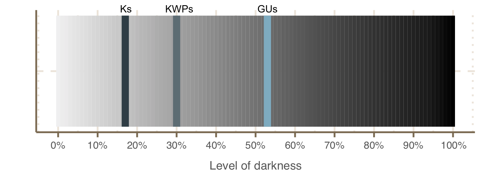
Schematic plot showing the level of darkness per cluster category.
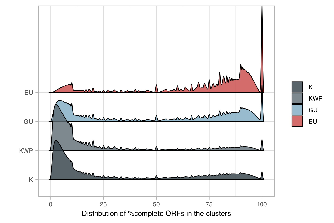
3. Cluster completeness
We retrieved the percentage of completeness for each cluster based on the percentage of complete ORFs (ORFs labeled by Prodigal [6] with “00” in the gene prediction step).
Scripts and description: The statistics were obtained passing to the script cluster_category_stats.r the refined set of clusters with partial information (marine_hmp_refined_cl.tsv.gz) and the correspondence cluster-category file (cl_ids_categ.tsv).
4. High quality (HQ) set of clusters
Using the completness information we retrieved a set of HQ clusters in terms of percentage of complete ORFs and the presence of a complete representative. The cluster representatives are those retrieved during the compositional validation step (see Cluster validation and refinement paragraph). To determine the clusters that are part of the HQ set, we first applied the broken-stick model [7] to determine a minimum required percentage of complete ORFs per cluster. Then, from the set of clusters above the threshold, we selected only the clusters with a complete representative.
Scripts and description: The set of HQ clusters is retrieved in the script cluster_category_stats.r.
High Quality clusters
| Category | HQ cluster | HQ ORFs | pHQ_orfs | pHQ_cl |
|---|---|---|---|---|
| K | 64,516 | 25105156 | 0.14583546 | 0.06143410 |
| KWP | 12,903 | 1349165 | 0.04408792 | 0.02040152 |
| GU | 82,671 | 8403393 | 0.15546789 | 0.07369436 |
| EU | 13,769 | 471820 | 0.14121033 | 0.10137011 |
As shown in the above table, the category with the highest percentage of HQ, i.e. complete, clusters is that of the EUs with 10% HQ clusters, followed by GUs and Ks. The KWPs have the least complete clusters and as showed in the previous section the highest level of (protein) disorder.
KWP eggNOG annotations grouped by COG category.
| COG category | n clusters |
|---|---|
| A | 818 |
| B | 447 |
| C | 29157 |
| D | 7993 |
| E | 42260 |
| F | 11595 |
| G | 35449 |
| H | 16241 |
| I | 13098 |
| J | 18358 |
| K | 15571 |
| L | 45348 |
| M | 51605 |
| N | 2858 |
| O | 21905 |
| P | 34841 |
| Q | 12070 |
| S | 138869 |
| T | 18448 |
| U | 12011 |
| V | 19284 |
| W | 410 |
| Y | 211 |
| Z | 1201 |
References
[1] M. Steinegger and J. Söding, “MMseqs2 enables sensitive protein sequence searching for the analysis of massive data sets.,” Nature biotechnology, vol. 35, no. 11, pp. 1026–1028, Nov. 2017.
[2] Hingamp, Pascal, Nigel Grimsley, Silvia G. Acinas, Camille Clerissi, Lucie Subirana, Julie Poulain, Isabel Ferrera, et al. 2013. “Exploring Nucleo-Cytoplasmic Large DNA Viruses in Tara Oceans Microbial Metagenomes.” The ISME Journal 7 (9): 1678–95.
[3] Dick, Jeffrey M. 2008. “Calculation of the Relative Metastabilities of Proteins Using the CHNOSZ Software Package.” Geochemical Transactions 9 (October): 10.
[4] Hausser, Jean, and Korbinian Strimmer. 2008. “Entropy Inference and the James-Stein Estimator, with Application to Nonlinear Gene Association Networks.” arXiv
[5] Perdigão, Nelson, Agostinho C. Rosa, and Seán I. O’Donoghue. 2017. “The Dark Proteome Database.” BioData Mining 10 (1): 1–11.
[6] Hyatt, Doug, Gwo-Liang Chen, Philip F. LoCascio, Miriam L. Land, Frank W. Larimer, and Loren J. Hauser. 2010. “Prodigal: Prokaryotic Gene Recognition and Translation Initiation Site Identification.” BMC Bioinformatics 11 (1): 119–119.
[7] Bennett, K. D. 1996. “Determination of the Number of Zones in a Biostratigraphical Sequence.” The New Phytologist 132 (1): 155–70.