Methods
The aim is to identify and aggregate clusters sharing detectable degree of homology, which are now split due to the limitations of the sequence similarity approach used by MMseqs2. To achieve this, we exploited distant homologies to create communities of clusters in the KNOWN space constrained by the domain architectures. The, using the information retrieved for the KNOWN space we partitioned the UNKNOWN space.
A non-redundant set of domain architectures. A larger proportion metagenomic data consists of fragmented ORFs, thus many of the domain architectures (DAs) we observed in the KNOWN space of fragmented ORFs could be part of a larger domain in a complete (or not) ORF. To minimise this effect, we identified DAs that could be part of a larger DA taking into account their topological order on the ORFs. In our data set, we had 29,341 different DAs. To speed up the process to identify if a DA could be a sub-DA of a larger one, we first calculated the pairwise string cosine distance (q-gram = 3) between pairs of DAs. This step allowed us to reduce the number of DA combinations to be screened, removing the DAs pairs that were too divergent. This was done conservatively with an applied a filter of a cosine distance < 0.9. We collapsed DAs that were fragments of larger DAs but taking into account the proportion of completed ORFs in each of the DAs. If a shorter DA has at least 75% of complete ORFs, is kept as an independent DA. After this filtering and collapsing step, we have 23,681 different DAs.
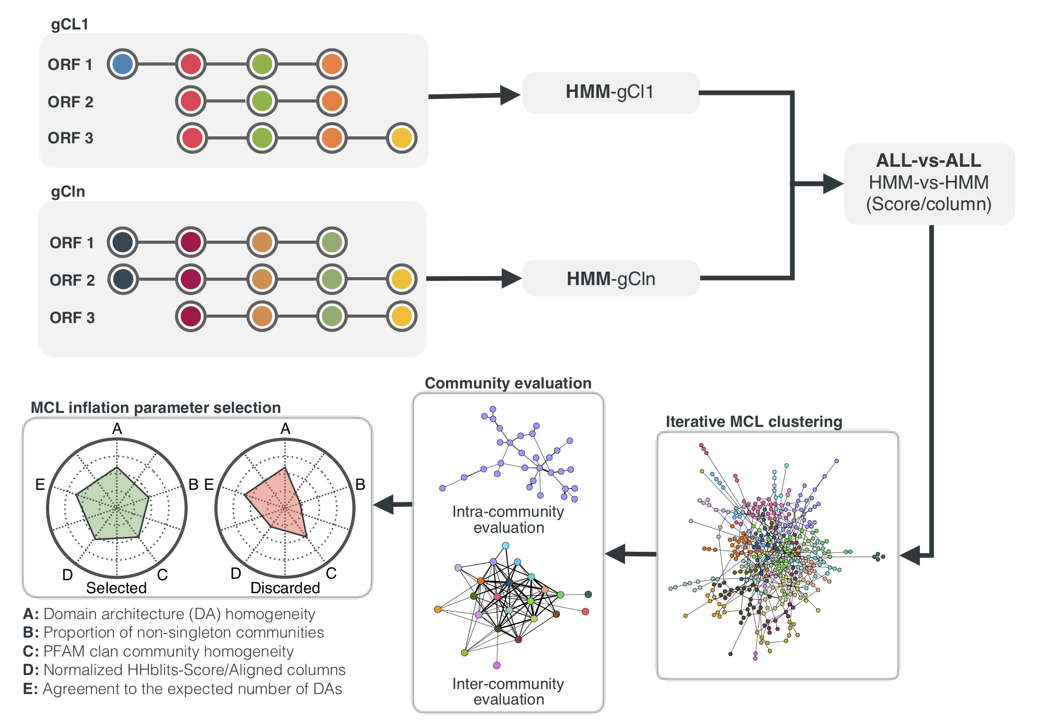
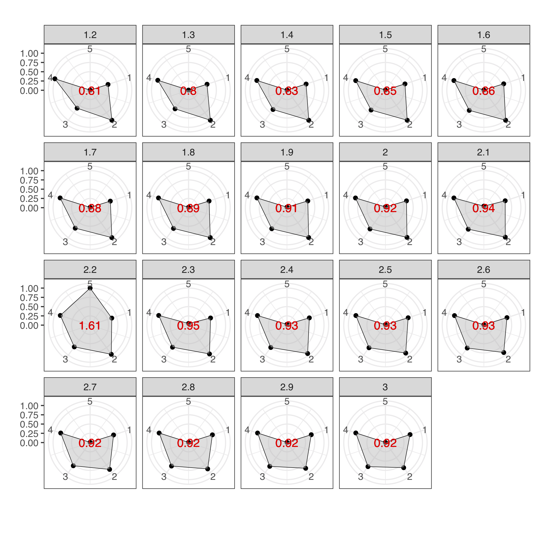
Graph inference. We used the HMMs of the KNOWN clusters to perform an all-vs-all HMM search with HHblits [1] (2 iterations and an e-value threshold of 1). We kept those pairs with a probability > 50% and a bidirectional coverage > 60%. Using the filtered results we created a network where we used the Score/aligned-columns as edge weights. Graph partitioning. To aggregate the clusters, we performed a community identification using the Markov Cluster Algorithm (MCL algorithm or clustering) [2], available at http://micans.org/mcl/ (v. 12-068). To identify the best inflation value we iterated through an interval of values starting from 1.2 until 3.0 in 0.1 incremental steps. For each of the inflation values, we explored the resulting communities in terms of five intra-/inter-community properties. We used the area of the radar plots were based on the area produced by the 5 variables allowed us a quick way to identify the best inflation value (Figure 2). As community properties, we explored: 1) The proportion of clusters with one single DA. For each community, we explored the consensus DA of each of the cluster members. To get the consensus DA of each cluster, we created a directed acyclic graph that encompassed the DAs of all ORFs in a cluster and obtained the intersection of those paths, keeping the most traversed path. Then for each MCL community, we performed the union of the consensus DAs of each cluster and decomposed the resulting network and counted the number of resulting components. 2) The proportion of communities with more than one member. The higher the MCL inflation value is, the larger the number of clusters is, and as a result of this, the number of communities with only one cluster increases. 3) The proportion of communities with a PFAM clan entropy equal to 0. 4) Intra HHblits Score/aligned-columns (normalised by the maximum value). 5) Number of communities (non-redundant set of DAs). The best inflation value corresponds to the radar plot with the largest area. Once determined the best inflation value, we added the missing clusters (nodes) to the MCL communities. We then used coverage, probability and Score/aligned-columns from the profile-vs-profile search results to find the best hits in a three-step approach: First, we checked if any of the not assigned clusters had any homology to the just classified ones using more relaxed filtering thresholds for the profile search results (probability ≥ 50% and coverage > 40%) and keeping just the best hits. Second, we found secondary relationships between the newly assigned clusters and the missing ones. And third, we ran the MCL algorithm on the missing clusters, using the identified best inflation value and we created new MCL communities. In the end, we collected and aggregated all communities. We repeated the whole process for the other categories (KWPs, GUs and EUs), with the exception that at the end we selected and applied the optimal inflation value found for the Ks.
Radar plots used to determine the best MCL inflation value for the partitioning of the Ks into cluster components. The plots were built using a combination of five variables: 1=proportion of clusters with 1 component and 2=proportion of clusters with more than 1 member, 3=clan entropy (proportion of clusters with entropy = 0), 4=intra hhblits score-per-column (normalised by the maximum value), and 5=number of clusters (related to the non-redundant set of DAs).
Scripts: community_inference.
Usage:
./community_inference/get_communities.R -c ${PWD}/community_inference/config.yml
Results
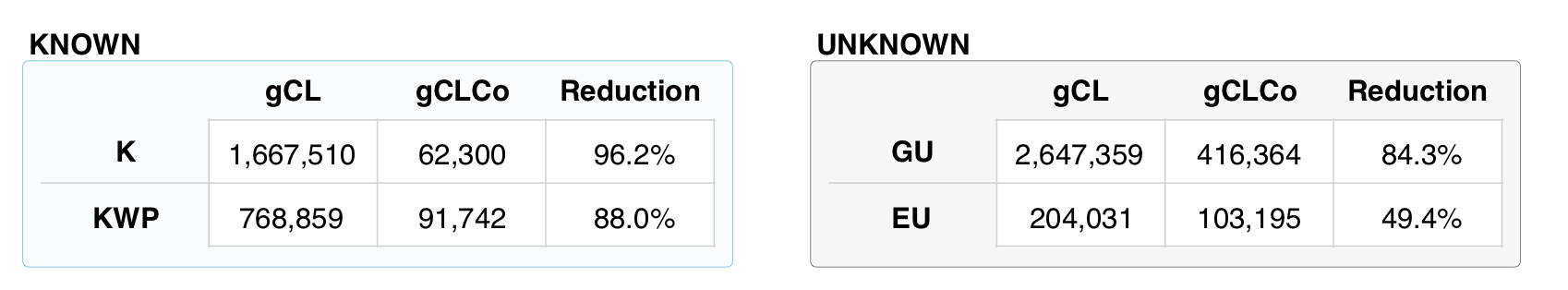
We found that a large proportion of Ks exhibited domain architecture redundancy between clusters. This may have been caused by the limitations of the clustering method used (based on sequence similarity) to detect distant homologies and the final threshold selected (30% of similarity). An inherent property of metagenomic data is that a large proportion of ORFs are fragmented. Therefore many of the DAs observed in the KNOWN space are part of fragmented ORFs which could be part of a larger DAs of another complete/partial ORF. To minimise this, we identified DAs that could be part of a larger ones. In our dataset, we had 29,341 different domain architectures, that after the filtering and collapsing steps were reduced to 23,681 different DAs. We determined an optimal inflation value of 2.2, corresponding to the radar plot with the largest area (Figure above), which is in agreement with the value empirically determined to be the optimal [2] (and close the software default of 2). The inference led to a set of 283,314 communities out of ~2.9M clusters. The numbers for each category are shown in the table below:
Overview of the workflow to aggregate GCs in communities. We inferred a gene cluster homology network using the results of an all-vs-all HMM gene cluster comparison with HHBLITS. The edges of the network are based on the HHblits-score/Aligned-columns. Communities are identified by an iterative screening of different MCL inflation parameters and evaluated using five different metrics that take into account the inter- and intra-community properties.
Comparison of the number of GCs and GCCs for each of the functional categories.
Number of communities, clusters and ORFs for each category.
| K | KWP | GU | EU | Total | |
|---|---|---|---|---|---|
| Communities | 24,181 | 64,938 | 146,100 | 48,095 | 283,314 |
| Clusters | 1,050,166 | 632,453 | 1,121,809 | 135,829 | 2,940,257 |
| ORFs | 172,147,128 | 30,601,694 | 54,052,275 | 3,341,257 | 260,142,354 |
Cluster communities validation
Methods
To prove the biological significance of the cluster communities, we explored how they distribute within the phylogeny of Proteorhodopsin (PR), a common and prevalent marine microbial functional protein. The hypothesis is that one community should encompass all PR reads and the clusters should subdivide the phylogeny by genus. We used the PR tree from Olson et al. [3].
The communities validation consisted in three steps:
1. We searched the proteorhodopsin HMM profiles against the K and KWP consensus sequences, using the hmmsearch program of the HMMER software (version 3.1b2) [4]. We filtered the results for coverage of ≥ 0.4 and e-value ≥ 1e-5. We extracted the amino acid sequences from each cluster that was recruited within the filtered results, and we used them as query sequences to be placed in the Olson et al. PR tree [3].
2. We placed the query sequences into the MicRhode [5] PR tree. We dereplicated the retrieved query sequences with CD-HIT (v4.6) [6], and we removed the remaining sequences with less than 100 amino acids using SEQKIT (v0.10.1) (Shen et al. 2016). Next, we calculated the best substitution model using the EPA-NG modeltest-ng (v0.3.5) [7] and we optimized the Olson et al. PR tree initial parameters and branch lengths using RAxML (v8.2.12) [8]. Afterwards, we performed an incremental alignment of the query sequences against the PR tree reference alignment using the PaPaRA (v2.5) software [9]. Then, we split the query alignment and the reference alignment using EPA-NG –split v0.3.5. We then combined the PR tree together with the related contextual data and the tree alignment, into a phylogenetic reference package using Taxtastic (v0.8.9), and we placed the query sequences in the tree using pplacer (v1.1.alpha19-0-g807f6f3) [10] with the option -p (–keep-at-most) set to 20. We grafted the PR tree with the query sequences using Guppy, tool that is part of pplacer.
3. In the end, we assigned PR Supercluster affiliation to query sequences. We assigned the PR Supercluster affiliation from Olson et al. [3] to the query sequences by calculating the Cophenetic Distance of the PR tree using the R packages ape (v5.3) [11] and refining the decision with a custom R script that used a combination of ape (v5.3) and phanghorn v2.5.3 [12].
Data visualization: We visualised the resulting data using the alluvial plot program from rawgraphs.io [13].
Scripts: community_validation.
Usage:
bash./scripts/place_PR.sh ${PWD}/all_sequences_names_to_extract.fasta ${PWD}/all_communities_2019-03-28-144550.tsv
In addition we explored how the cluster communities and the subset of high quality (HQ) clusters and their communties distribute among a bacterial set of ribosomal protein families. For the analysis we used the set 16 ribosomal proteins used in Méheust et al. [14] (ribo_markers.tsv) in combination with the collection of bacterial single copy genes (scg) of Anvi’o [15], that can be downloaded from here.
Script: The ribosomal protein analysis was performed using the R script cl_comm_ribo_prot.r. The output files: “ribo_com_cl.tsv” and “ribo_com_cl_hq.tsv” can be visualised/plotted usaing the RawGraphs visualization framework.
Results
Olson et al. [3] phylogenetically analysed PRs in the sunlit ocean and grouped them into clades called Superclusters. We found that our clusters resolve the PR’s Superclusters, as shown in the figure below. We observed one large K community encompassing the 99% of the PR annotated ORFs. All the superclusters are represented in the K community, with the only exception of 20 ORFs annotated to PR supercluster I, mostly viral, that fall into two GU communities (5 GU clusters) .
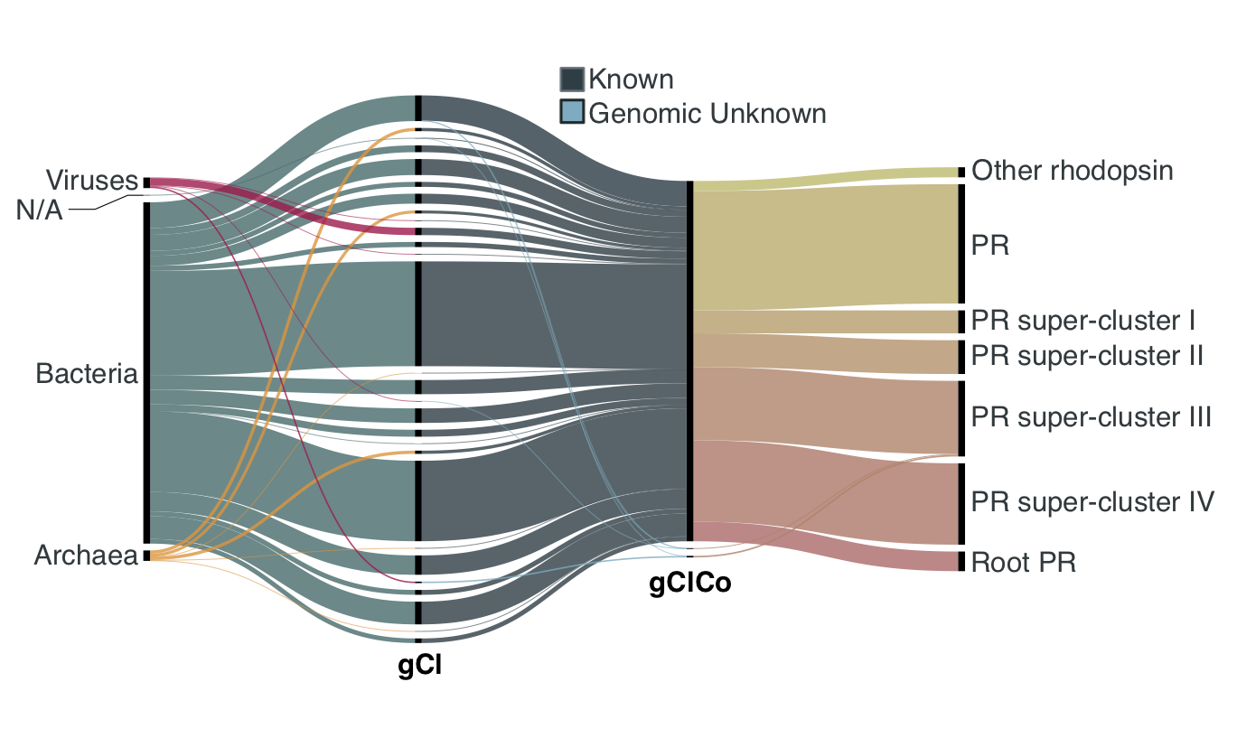
Validation of the GCCs inference based on the environmental genes annotated as proteorhodopsins. Ribbons in the alluvial plot are genes, and each stacked bar corresponds (from left to right) to the (1) gene taxonomic classification at domain level, (2) GC membership, (3) GCC membership and (4) MicRhoDE operational classification.
Number of genes, clusters and communities annotated to PR
| Genes | Clusters | Communities |
|---|---|---|
| 12,184 | 64 | 3 |
The distribution of the cluster communitites among 16 bacterial ribosomal protein families reflects the fragmented nature of metagenoic data. Because ribosomal proteins are highly conserved, we expect one protein family per ribosomal subunit. However, we observe the same ribosomal protein falling in different communities and this is likely due to the fragmented nature of metagenomic ORFs. In fact, this effect almost disappear when we subset for the communities containing only HQ clusters (high percentage of complete ORFs), as shown in the next figure:
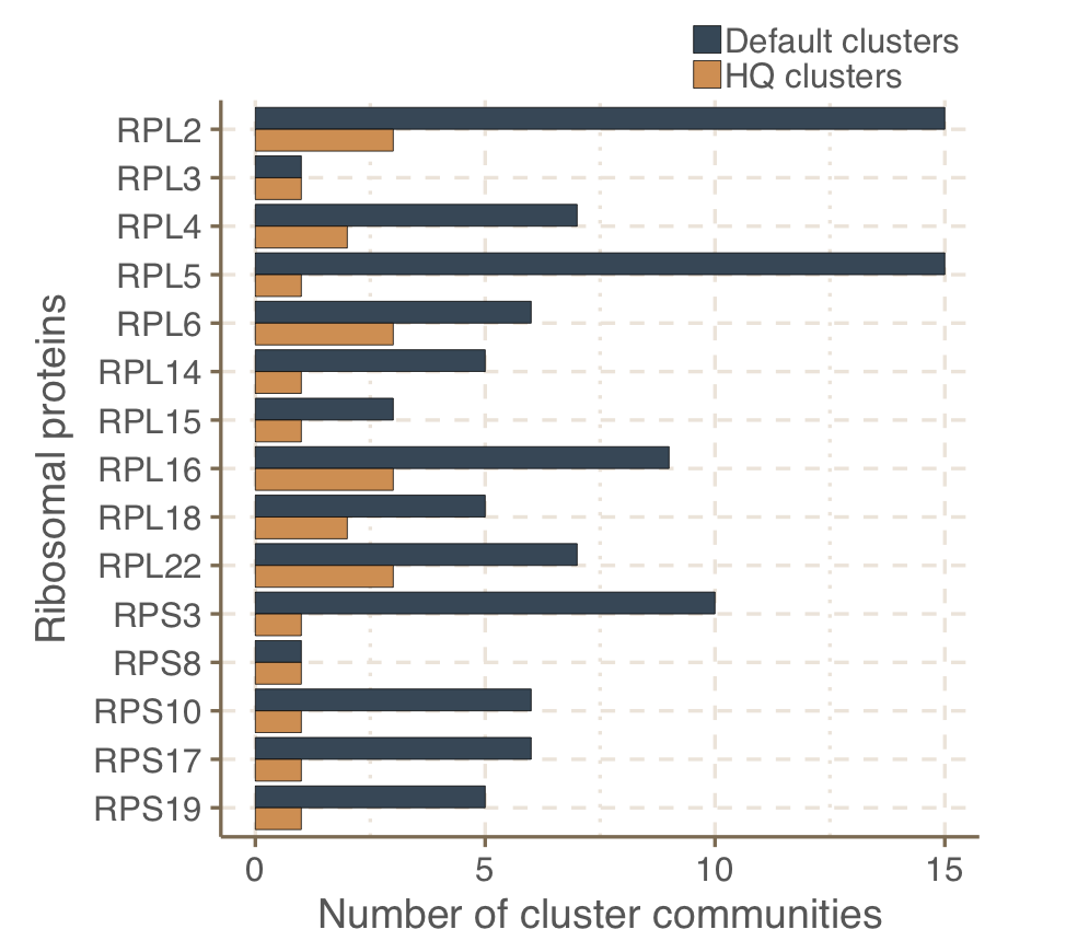
Validation of the GCCs inference based on ribosomal proteins based on standard and high-quality GCs.
Number of genes, clusters and communities annotated to ribosomial proteins
| Genes | Clusters | Communities | |
|---|---|---|---|
| All clusters | 781,579 | 1,843 | 98 |
| HQ clusters | 1,687 | 145 | 26 |
Communities inference methods comparison
We compared our community inference method with the one used by Méheust et al. [14].
Methods The cluster community inference was validated in comparison to the approach used by Méheust et al. (2019), using the ribosomal protein families as reference. The approach used by Méheust et al. is very similar to ours. They first clustered the genes using MMseqs2 (version 9f493f538d28b1412a2d124614e9d6ee27a55f45), performing an all-vs.-all search (e-value: 0.001, sensitivity: 7.5, and cover: 0.5). The search results were used to build a sequence similarity network that was then partitioned, using the greedy set cover algorithm from MMseqs2, into what they defined as subfamilies. Their subfamilies correspond to our gene clusters. The subfamilies were then aggregated into families, based on remote homologies. Their families correspond to our gene cluster communities. For the aggregation they compared the subfamilies HMM profiles using hhblits from the HHpred suite. From this search they selected the subfamilies with hhblits-probability ≥95% and coverage ≥0.50. They used a similarity score (probability × coverage) as weight for the search sequence similarity network. This network was then partitioned using the Markov CLustering algorithm (MCL), with 2.0 as the inflation parameter.
The main differences with our method:
- We used the score/cols (hhblits search score over number of aligned columns) as edge weight for the sequence similarity network.
- We didn’t use a default MCL inflation parameter for the partitioning of the sequence similarity network. We tested several values on the set of Known clusters. The best inflation value was then determined using the combination of different metrics, including the Pfam domain architecture composition of our gene clusters.
The cluster communities were filtered for those annotated to the 16 ribosomal proteins used in Méheust et al., and those contained in the collection of bacterial single-copy genes of Anvi’o10, that can be downloaded from (https://github.com/merenlab/anvio/blob/master/anvio/data/hmm/Bacteria_71/genes.txt). The genes contained in this community subset, were processed using the approach proposed by Méheust et al. The results were then compared with those obtained in this paper using the functions of the R package aricode (https://github.com/jchiquet/aricode), which allow comparisons between clustering methods.
Scripts: The code used for this analysis can be found in cl_comm_ribo_prot.r.
Results The clustering approach proposed in this paper was compared to the method used by Méheust et al. and validated using a set of ribosomal proteins. Overall, our approach generated less cluster communities as can be observed in the figure below. Our clustering was found closer to the “ground truth” represented by the ribosomal protein families compared to the partitioning proposed by Méheust et al. The results from the comparison between the two clustering approaches and the ribosomal protein reference are reported in the table below.
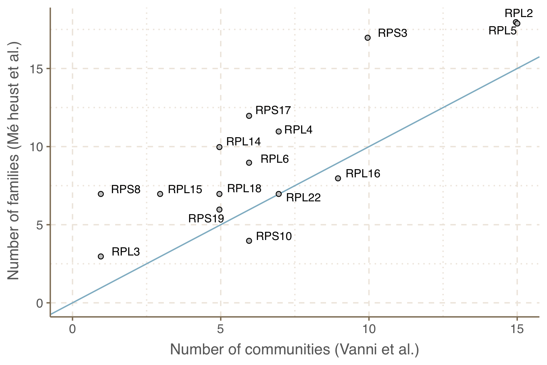
Number of communities within ribosomal protein families, comparison between the number generated by our approach and the number obtained by Méheust et al.
| Vanni et al. vs Meheust et al. | Vanni et al. vs ribosomal families | Meheust et al. vs ribosomal families | |
|---|---|---|---|
| ARI | 0.915 | 0.944 | 0.906 |
| AMI | 0.928 | 0.916 | 0.878 |
| NVI | 0.101 | 0.0858 | 0.124 |
| NID | 0.0717 | 0.0841 | 0.122 |
| NMI | 0.928 | 0.916 | 0.878 |
</div>
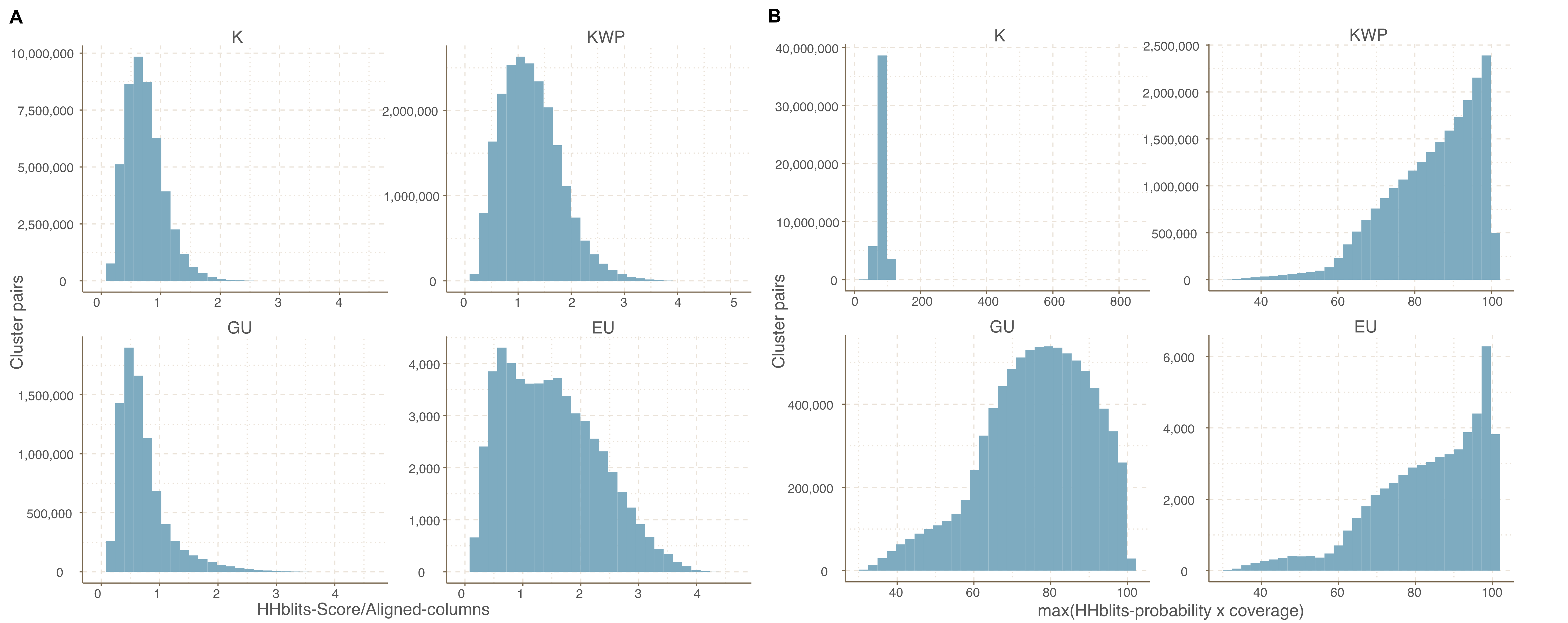
Cluster pairs distribution based on the metrics used to weight the gene cluster HMM-HMM homology network. (A) HHblits-Score/Aligned-columns (Vanni et al.). (B) maximum(HHblits-probability x coverage) (Méheust et al.).
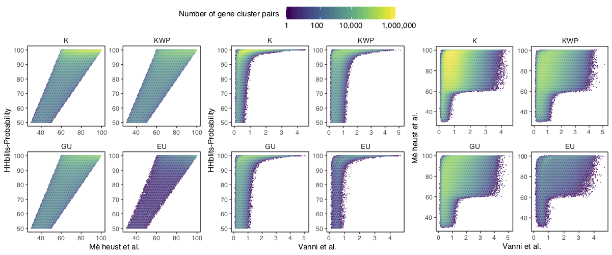
Determination of the edge-weight metrics for the GC HMM-HMM homology network. We tested the metrics used in Méheust et al. and in this paper (Vanni et al.). The correlations between metrics are shown per functional category. The metric used by Méheust et al. corresponds to the maximum(HHblits-probability x coverage). The metric applied in this paper is the HHblits-Score/Aligned-columns. (A) Correlation between the Méheust et al. metric and the HHblits-probability. (B) Correlation between the Vanni et al. metric and the HHblits-probability. (C) Correlation between the Vanni et al. and the Méheust et al. metrics.
References
[1] M. Remmert, A. Biegert, A. Hauser, and J. Söding, “HHblits: lightning-fast iterative protein sequence searching by HMM-HMM alignment.,” Nat Methods, Nov. 2011.
[2] van Dongen, Stijn van, and Cei Abreu-Goodger. 2012. “Using MCL to Extract Clusters from Networks.” In Bacterial Molecular Networks: Methods and Protocols, edited by Jacques van Helden, Ariane Toussaint, and Denis Thieffry, 281–95. New York, NY: Springer New York.
[3] Olson, Daniel K., Susumu Yoshizawa, Dominique Boeuf, Wataru Iwasaki, and Edward F. DeLong. 2018. “Proteorhodopsin Variability and Distribution in the North Pacific Subtropical Gyre.” The ISME Journal 12 (4): 1047–60.
[4] Finn, R. D., J. Clements, and S. R. Eddy. 2011. “HMMER Web Server: Interactive Sequence Similarity Searching.” Nucleic Acids Research 39 (suppl): W29–37.
[5] Boeuf, Dominique, Stéphane Audic, Loraine Brillet-Guéguen, Christophe Caron, and Christian Jeanthon. 2015. “MicRhoDE: A Curated Database for the Analysis of Microbial Rhodopsin Diversity and Evolution.” Database: The Journal of Biological Databases and Curation 2015 (August).
[6] Li, W., and A. Godzik. 2006. “Cd-Hit: A Fast Program for Clustering and Comparing Large Sets of Protein or Nucleotide Sequences.” Bioinformatics 22 (13): 1658–59.
[7] Barbera, Pierre, Alexey M. Kozlov, Lucas Czech, Benoit Morel, Diego Darriba, Tomáš Flouri, and Alexandros Stamatakis. 2019. “EPA-Ng: Massively Parallel Evolutionary Placement of Genetic Sequences.” Systematic Biology 68 (2): 365–69.
[8] Stamatakis, Alexandros. 2014. “RAxML Version 8: A Tool for Phylogenetic Analysis and Post-Analysis of Large Phylogenies.” Bioinformatics 30 (9): 1312–13.
[9] Berger, Simon A., and Alexandros Stamatakis. 2012. “PaPaRa 2.0: A Vectorized Algorithm for Probabilistic Phylogeny-Aware Alignment Extension.” Heidelberg Institute for Theoretical Studies
[10] Matsen, Frederick A., Robin B. Kodner, and E. Virginia Armbrust. 2010. “Pplacer: Linear Time Maximum-Likelihood and Bayesian Phylogenetic Placement of Sequences onto a Fixed Reference Tree.” BMC Bioinformatics 11 (October): 538.
[11] Paradis E. & Schliep K. 2018. ape 5.0: an environment for modern phylogenetics and evolutionary analyses in R. Bioinformatics 35: 526-528.
[12] Schliep, Klaus Peter. 2011. “Phangorn: Phylogenetic Analysis in R.” Bioinformatics 27 (4): 592–93.
[13] Mauri, Michele, Tommaso Elli, Giorgio Caviglia, Giorgio Uboldi, and Matteo Azzi. 2017. “RAWGraphs: A Visualisation Platform to Create Open Outputs.” In Proceedings of the 12th Biannual Conference on Italian SIGCHI Chapter, 28. ACM.
[14] Méheust, Raphaël, David Burstein, Cindy J. Castelle, and Jillian F. Banfield. 2019. “The Distinction of CPR Bacteria from Other Bacteria Based on Protein Family Content.” Nature Communications 10 (1): 4173.
[15] Murat, E. A., Özcan C. Esen, Christopher Quince, Joseph H. Vineis, Hilary G. Morrison, Mitchell L. Sogin, and Tom O. Delmont. 2015. “Anvi’o: An Advanced Analysis and Visualization Platform for ‘omics Data.” PeerJ 3 (October): e1319.