Gene Cluster validation

An evaluation of the clustering is necessary to compare the functional homogeneity of the sequences within the same cluster [1]. The ORF clusters represent the basis of all the further analyses; hence we need to ensure a good clustering quality in terms of high intra-cluster homogeneity.

Methods

We proceeded with the validation of both annotated and not annotated clusters following two different strategies: i) we evaluated clusters homogeneity at the sequence level, based on an estimation of the homologous and non-homologous relations between sequences in a protein multiple sequence alignment; and ii) we measured the functional homogeneity within the clusters, based on the member’s functional annotations. A detailed description of both methods follows:

A) Compositional homogeneity
To identify improper/incongruous sequences inside each cluster, we performed a multiple sequence alignment (MSA) within each cluster, using the FAMSA fast multiple alignments program [2] (version 1.1). To evaluate the MSAs of clusters with a size ranging between 10 and 1K ORFs, we then used LEON-BIS [3], a method that allows the accurate detection of conserved regions in multiple sequence alignments, via Bayesian statistics, identifying the non-homologous sequences with respect to the cluster representative. LEON-BIS proved to be too computationally expensive in processing clusters with more than 1K ORFs, thus we proceeded with OD-SEQ [4], a tool that identifies outliers ORFs based on their average distance from the other sequences. In the end, We applied the broken-stick model [5] to the detected incongruous ORFs distribution in the clusters to determine the cut-off number above which we classified a cluster as “bad”. In parallel we applied PARASAIL [6] (version 2.1.5), a C library for global, semi-global and local alignments, to retrieve the ‘all vs all’ similarities (pairwise similarities) within each cluster and build the correspondent sequence similarity network (SSN), i.e. a homology graph where the nodes are the ORFs and the edges the similarities). We thus trimmed the SSN using an algorithm that removes edges while maintaining the structural integrity, and we used a measure of centrality (specifically the eigenvector centrality) to refine the cluster representative selection and identify a proper representative sequence for each cluster (more details in the next paragraph/supplementary).

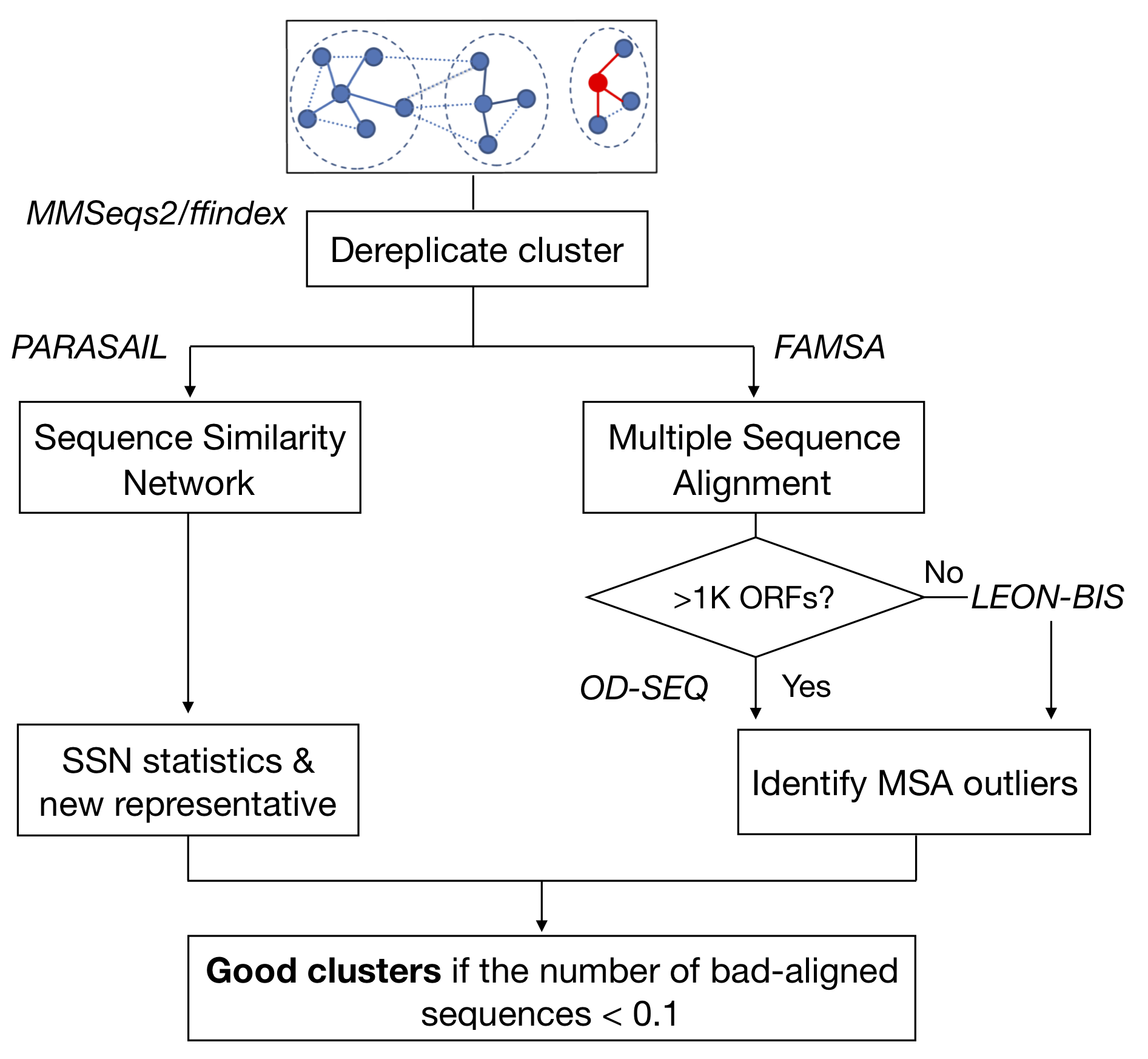Figure 1. Cluster compositional homogeneity validation scheme.

B) Functional homogeneity
Since our predicted ORFs can have multiple (multi-domain) annotations, in different orders, we investigated the functional composition of the annotated clusters applying a combination of text mining and Jaccard similarity. As text mining technique we used Shingling, a method commonly used in the field of language processing to represent documents as sets. A k-shingle is a consecutive set of k words. Once transformed the protein domain annotations of each cluster’s member into shingle sets, we calculated the Jaccard similarity between sets of shingles as the ratio between distinct shared shingles and distinct unshared shingles between two members. The median Jaccard similarity score was calculated for each cluster and scaled by the percentage of annotated members. Since different Pfam domains can be grouped into the same clan (“A collection of related Pfam entries. The relationship may be defined by similarity of sequence, structure or profile-HMM.”), we decided to consider completely homogeneous those clusters annotated to the same clan. In addition Pfam contains both C-terminal, N-terminal and few times the M-(middle) domains of some proteins, hence (since we are dealing with fragmented ORFs) we decided to consider completely homogeneous those clusters annotated to different domains of the same protein.

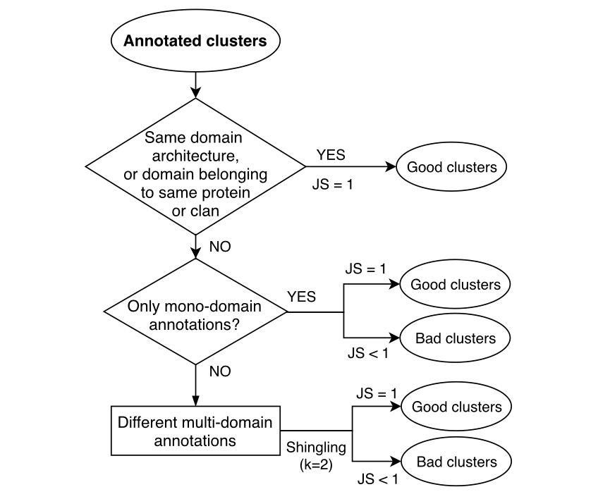Figure 2. Cluster functional homogeneity validation: general scheme.

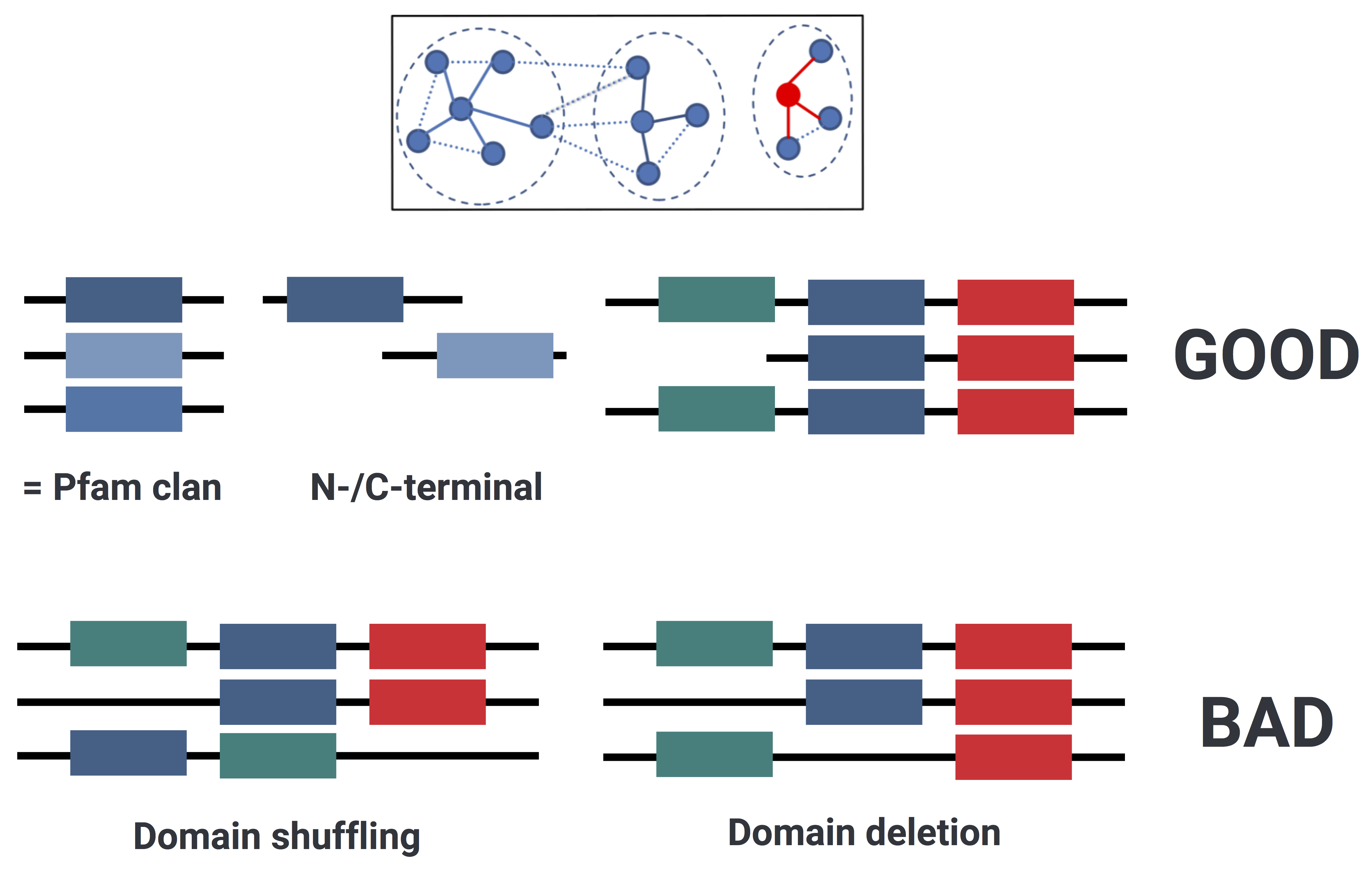
Figure 3. Cluster functional homogeneity validation: illustration of different possible cases inside the clusters.

More in detail, the evaluation of the functional homogeneity is based on the following decisions:

Figure 4. Functional homogeneity decision tree

1. If all the cluster members are annotated to the same Pfam domain (“Homog_pf”) Shingling is not applied and the Jaccard similarity index is calculated, and scaled for the percentage of annotated members.

2. If all the cluster members are annotated to different Pfam domains belonging to the same clan (“Homo_clan”) Shingling is not applied and the Jaccard similarity index is calculated, and scaled for the percentage of annotated members.

3. If the annotations (domains - clans) are not completely homogeneous, we look for different terminal (or middle) domains of the same protein.

   • If all the cluster members are terminal/middle domains of the same protein (“Homog_pf_term”) Shingling is not applied and the Jaccard similarity index is calculated, and scaled for the percentage of annotated members.

In the case, that any of the conditions is true, we will check if the cluster contains only mono-domain annotations, or also multi-domain?

1. ”Mono”: Shingling is not applied and the Jaccard similarity index is calculated, both for Pfam domains (“Mono_pf”) and clans (“Mono_clan”) annotations, and scaled for the percentage of annotated members. The higher index (between domains and clans) is reported.

2. If a cluster contains also multi-domain annotations, does it contains also ORFs with mono-domain annotations?

   • If yes: The Jaccard similarity index is calculated for the ORFs with mono-annotations (“Singl_pf” or “Singl_clan”) and scaled by their proportion. The domains/clans of the members with multi-annotations (“Multi_pf” or “Multi_clan”) are transformed into shingle sets (k=2), the Jaccard similarity is calculated on them and scaled by the proportion of ORFs with multi-annotations.

   • If no: The domains/clans of the clusters with multi-annotations (“Multi_pf” or “Multi_clan”) are transformed into shingle sets (k=2), the Jaccard similarity index is calculated on them and scaled by the proportion of ORFs with multi-annotations (i.e. the annotated ORFs in the cluster).

The overall higher Jaccard indexes (between domains and clans) are chosen/reported.

Results

The compositional homogeneity evaluation of the clusters confirmed a good cluster quality at the sequence level. Of the ∼3 million clusters 249,506 (8%) contain a rejected sequence (i.e., bad-aligned sequence). We identified the proportion of rejected sequences that defines a cluster as “bad” at 10% of the ORFs in a cluster. About 46K (1.9%) clusters resulted classified as “bad”.

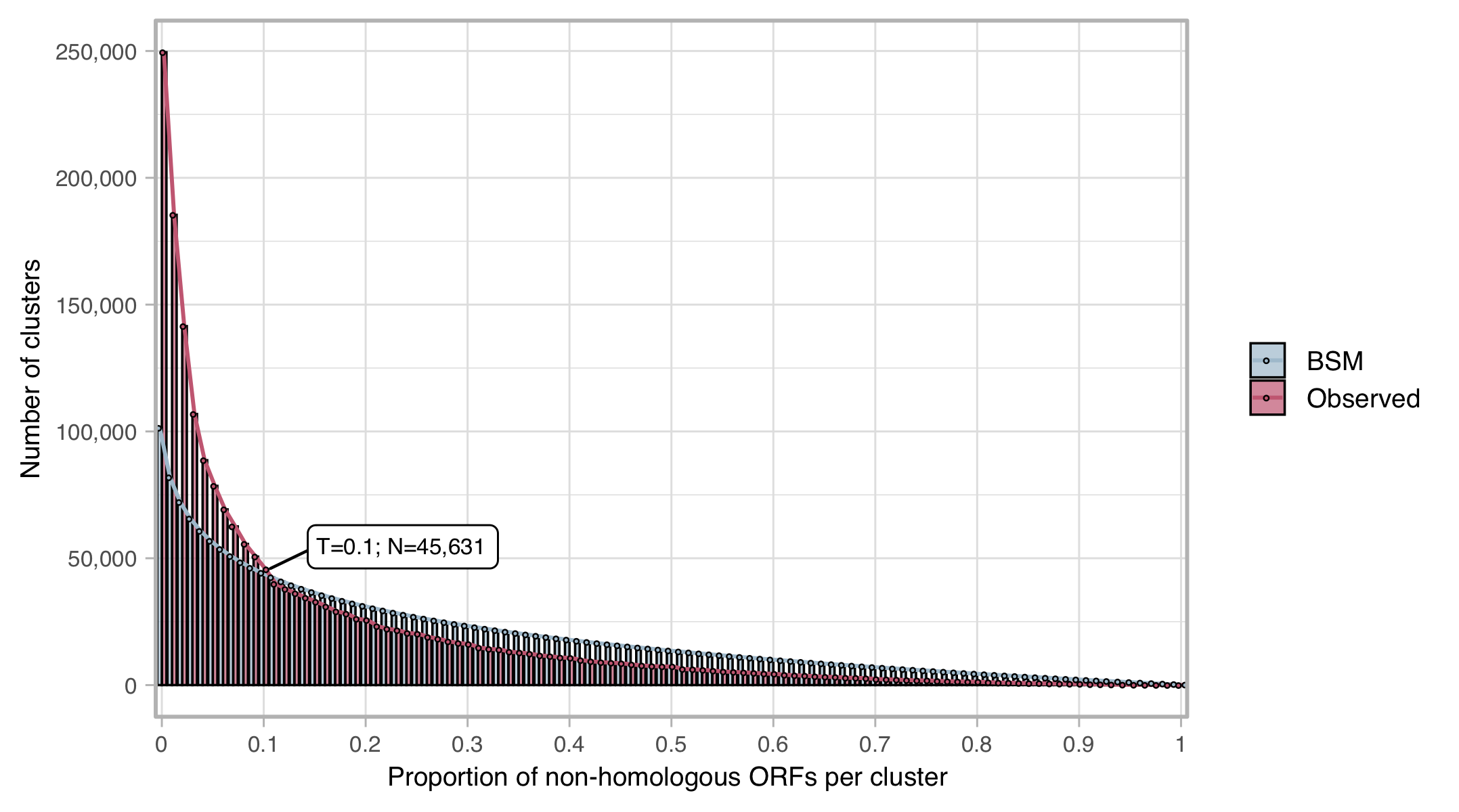Figure 5. Proportion of bad-aligned/non-homologous ORFs detected within each cluster MSA. Distribution of observed values compared with those of the Broken-stick model. The threshold was determined at 10% non-homologous ORFs per cluster.

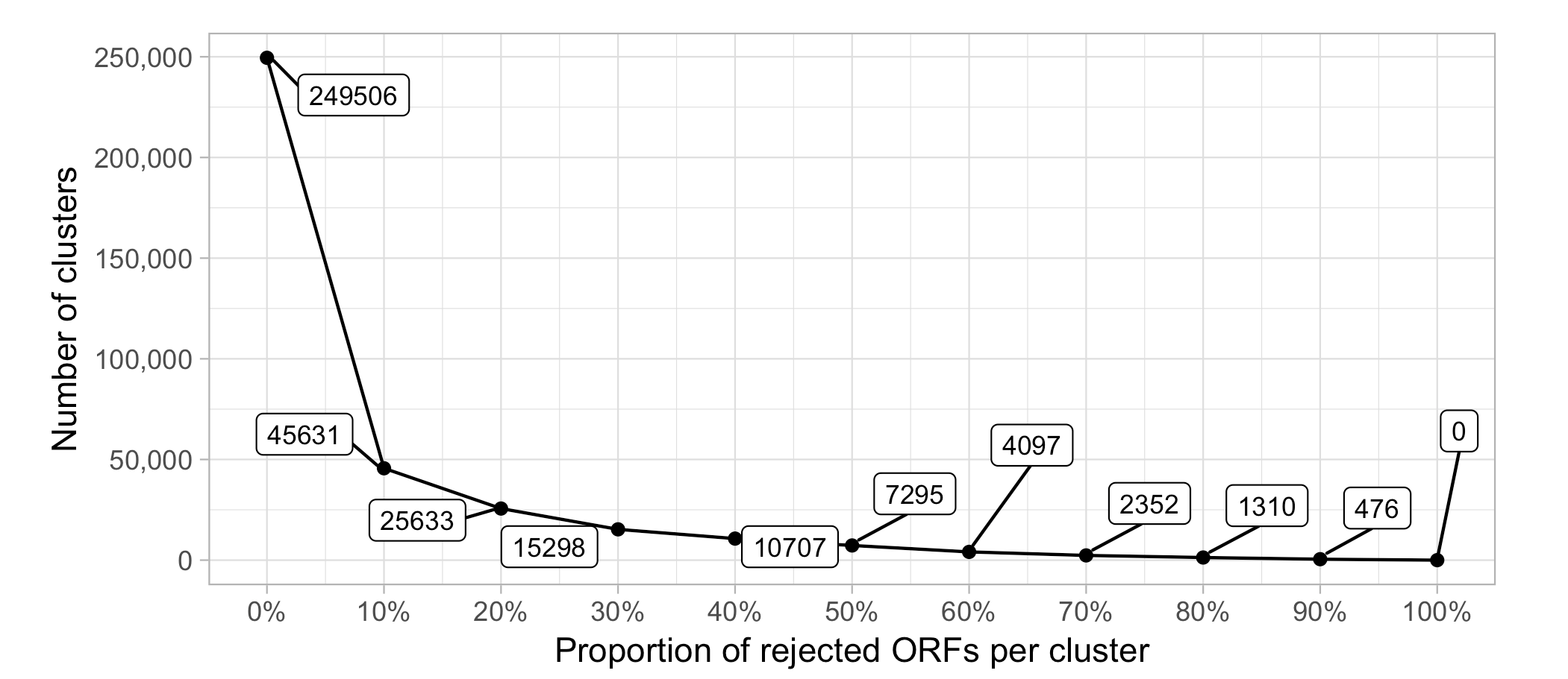Figure 6. Number of clusters as a function of the proportion of rejected ORFs per cluster

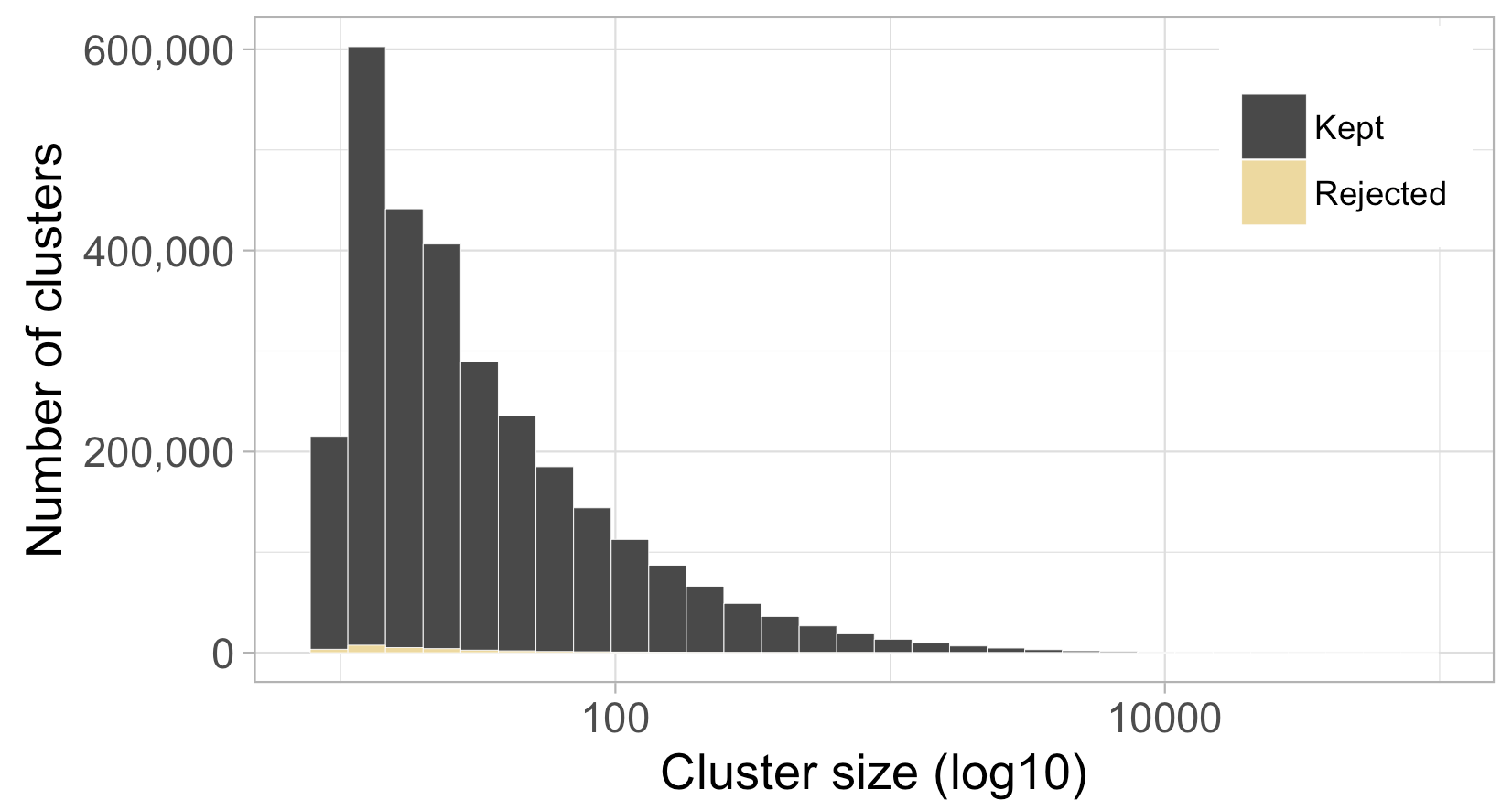Figure 7. Size distribution of the kept and rejected clusters

We observed an overall high functional homogeneity for the set of annotated clusters. Only 1% of the annotated clusters reported a Jaccard similarity index < 1.

The combination of the results of both cluster evaluations led to a set of 2,946,845 (98.1%) “good” clusters and 57,052 (1.9%) “bad” clusters. The number of ORFs in the two sets is shown in the following table.

Table 1. Number “good” and “bad” clusters defined after the validation and number of ORFs in them.

Good Clusters	Bad Clusters
2,946,845 (98.1%)	57,052 (1.9%)
Good Clusters ORFs	Bad Clusters ORFs
263,022,636 (98%)	5,445,127 (2%)

The proportion of rejected sequences appears to decrease at the increasing of the intra-cluster average similarity, as shown in the plots of the next figure.

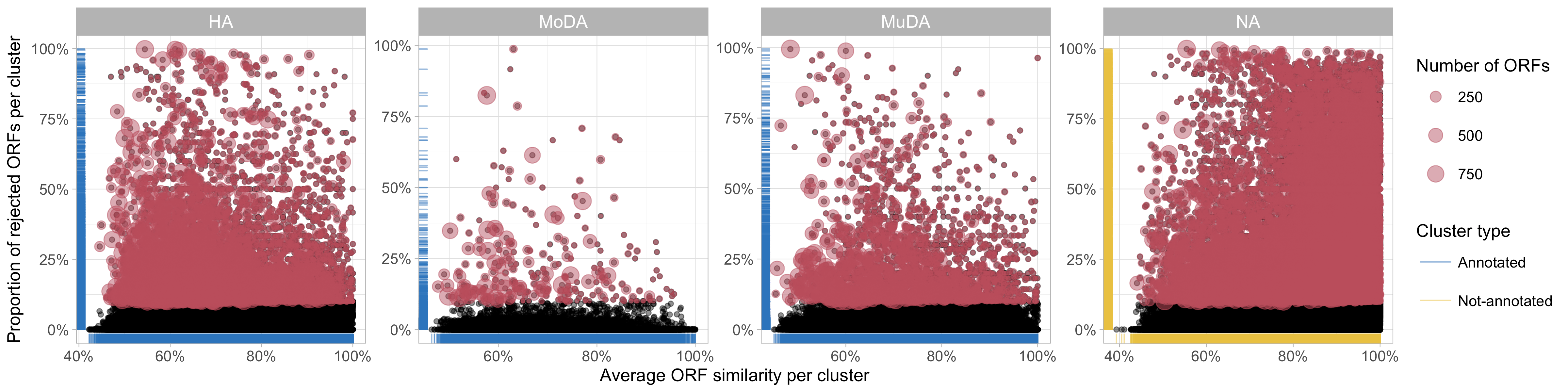Figure 8. Relationship between the proportion of rejected ORFs identified and the average ORF similarity within each cluster (In red rejected clusters).

We don’t observe a particular correlation between the number of bad-aligned ORFs and the annotation status of the clusters.

We compared the two validation steps for the set of annotated clusters, and we found that they agree in the identification of homogeneous and non-homogeneous clusters. As reported in the following Table, only 2% of the annotated clusters (and 2% of their ORFs) show discordant results between the two validations.

Table 1. Cluster validation result comparison.

CLUSTERS	Functional BAD	Functional GOOD	Not annotated clusters
Compositional BAD	337	9,006	36,288
Compositional GOOD	11,421	995,160	1,951,685

ORFs	Functional BAD	Functional GOOD	Not annotated clusters
Compositional BAD	19,956	990,903	1,188,266
Compositional GOOD	3,246,002	177,176,680	85,845,956

---